Reciprocal Gamma function
In mathematics, the reciprocal Gamma function is the function
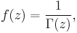
where  denotes the Gamma function. Since the Gamma function is meromorphic and nonzero everywhere in the complex plane, its reciprocal is an entire function. The reciprocal is sometimes used as a starting point for numerical computation of the Gamma function, and a few software libraries provide it separately from the regular Gamma function.
Karl Weierstrass called the reciprocal Gamma function the "factorielle" and used it in his development of the Weierstrass factorization theorem.
Contents |
Taylor series
Taylor series expansion around 0 gives
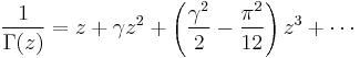
where  is the Euler–Mascheroni constant. For k > 2, the coefficient ak for the zk term can be computed recursively as
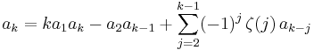
where ζ(s) is the Riemann zeta function. For small values, this gives the following values:
| k |  |
|---|---|
| 1 | 1.0000000000000000000000000000000000000000 |
| 2 | 0.5772156649015328606065120900824024310422 |
| 3 | −0.6558780715202538810770195151453904812798 |
| 4 | −0.0420026350340952355290039348754298187114 |
| 5 | 0.1665386113822914895017007951021052357178 |
| 6 | −0.0421977345555443367482083012891873913017 |
| 7 | −0.0096219715278769735621149216723481989754 |
| 8 | 0.0072189432466630995423950103404465727099 |
| 9 | −0.0011651675918590651121139710840183886668 |
| 10 | −0.0002152416741149509728157299630536478065 |
| 11 | 0.0001280502823881161861531986263281643234 |
| 12 | −0.0000201348547807882386556893914210218184 |
| 13 | −0.0000012504934821426706573453594738330922 |
| 14 | 0.0000011330272319816958823741296203307449 |
| 15 | −0.0000002056338416977607103450154130020573 |
| 16 | 0.0000000061160951044814158178624986828553 |
| 17 | 0.0000000050020076444692229300556650480600 |
| 18 | −0.0000000011812745704870201445881265654365 |
| 19 | 0.0000000001043426711691100510491540332312 |
| 20 | 0.0000000000077822634399050712540499373114 |
| 21 | −0.0000000000036968056186422057081878158781 |
| 22 | 0.0000000000005100370287454475979015481323 |
| 23 | −0.0000000000000205832605356650678322242954 |
| 24 | −0.0000000000000053481225394230179823700173 |
| 25 | 0.0000000000000012267786282382607901588938 |
| 26 | −0.0000000000000001181259301697458769513765 |
| 27 | 0.0000000000000000011866922547516003325798 |
| 28 | 0.0000000000000000014123806553180317815558 |
| 29 | −0.0000000000000000002298745684435370206592 |
| 30 | 0.0000000000000000000171440632192733743338 |
Contour integral representation
An integral representation due to Hermann Hankel is

where C is a path encircling 0 in the positive direction, beginning at and returning to positive infinity with respect for the branch cut along the positive real axis. According to Schmelzer & Trefethen, numerical evaluation of Hankel's integral is the basis of some of the best methods for computing the Gamma function.
Integral along the real axis
Integration of the reciprocal Gamma function along the positive real axis gives the value
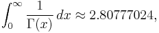
which is known as the Fransén–Robinson constant.
See also
References
- Thomas Schmelzer & Lloyd N. Trefethen, Computing the Gamma function using contour integrals and rational approximations
- Mette Lund, An integral for the reciprocal Gamma function
- Milton Abramowitz & Irene A. Stegun, Handbook of Mathematical Functions with Formulas, Graphs, and Mathematical Tables
- Eric W. Weisstein, Gamma Function, MathWorld